- 데이터 핸들링
- 함수
- 기술 통계 & Visualization
R 강의
두번째 시간
김형준
Data Analyst
Contents
주의 사항
a = 1:2; b = 3:5; c = 2:5
cbind(a,b)
## Warning: number of rows of result is not a multiple of vector length (arg
## 1)
##      a b
## [1,] 1 3
## [2,] 2 4
## [3,] 1 5
rbind(a,c)
##   [,1] [,2] [,3] [,4]
## a    1    2    1    2
## c    2    3    4    5
함수
- IF 문
if (.Platform$OS.type == "unix") {
    path_dir = "A"
} else {
    path_dir = "B"
    windowsFonts(NanumGothic=windowsFont("NanumGothic"))
}
- library('foo') stops when foo was not installed
- require() is basically try(library()) 보통 library 를 처음에 위치, require -> 저 아래에서 실행할 때 오류
if (!require("dplyr")) {
  install.packages("dplyr")
}
- FOR 문
for (i in 1:3)
{
print(i)
    for (j in 1:3)
        print(j)
}
- Function \[\sqrt{(a^2+b^2)}\]
norm_op = function(a,b)
{
    norm = a^2 + b^2
    return(sqrt(norm))
}

norm_op(1,3)  == sqrt(10)
## [1] TRUE
library("hflights")
dim(hflights); nrow(hflights); ncol(hflights)
## [1] 227496 21
## [1] 227496
## [1] 21
colnames(hflights); #range(rownames(hflights))
##  [1] "Year"              "Month"             "DayofMonth"
##  [4] "DayOfWeek"         "DepTime"           "ArrTime"
##  [7] "UniqueCarrier"     "FlightNum"         "TailNum"
## [10] "ActualElapsedTime" "AirTime"           "ArrDelay"
## [13] "DepDelay"          "Origin"            "Dest"
## [16] "Distance"          "TaxiIn"            "TaxiOut"
## [19] "Cancelled"         "CancellationCode"  "Diverted"
기술 통계
자료의 특성을 표, 그림, 통계량 등을 사용하여 쉽게 파악할 수 있도록 정리요약
- 평균 (mean) / 중앙값 (median) / 합계 (sum)
- 분산 (variance) / 표준편차 (sd)
- 범위 (range)
- 상관 (cor)
mean(hflights[,"DepTime"]) # 평균-> NA
## [1] NA
mean(hflights[,"DepTime"],na.rm=T) # 평균(missing 제거)
## [1] 1396
sapply(hflights,is.numeric) ## Numeric or not
sapply(hflights[,sapply(hflights,is.numeric)],mean)
sapply(hflights[,sapply(hflights,is.numeric)],function(x) mean(x, na.rm=T))
boxplot(hflights[,sapply(hflights,is.numeric)])

col_sel = colnames(hflights)[sapply(hflights,is.numeric)]
boxplot(hflights[,col_sel], xaxt="n")
text(x =  1:length(col_sel), y = par("usr")[3] - 1, srt = 90, adj = 1,
     labels = col_sel, xpd=T)

library("reshape")
hflights_df = hflights[,sapply(hflights,is.numeric)]
hflights_df[,"id"] = 1:nrow(hflights_df)
#head(hflights_df)
hflights_df_m = melt(hflights_df,id="id")
library(ggplot2)
ggplot(hflights_df_m) +
geom_boxplot(aes(x=variable, y=value))+
xlab("")+
theme(text=element_text(size=10),
axis.text.x = element_text(angle = 90, size = 14, hjust=1))
print(paste("# of Missing is", sum(is.na(hflights_df))))
## Warning: Removed 25755 rows containing non-finite values (stat_boxplot).
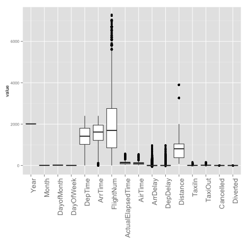
## [1] "# of Missing is 25755"
summary
summary(iris)
##   Sepal.Length   Sepal.Width    Petal.Length   Petal.Width
##  Min.   :4.30   Min.   :2.00   Min.   :1.00   Min.   :0.1
##  1st Qu.:5.10   1st Qu.:2.80   1st Qu.:1.60   1st Qu.:0.3
##  Median :5.80   Median :3.00   Median :4.35   Median :1.3
##  Mean   :5.84   Mean   :3.06   Mean   :3.76   Mean   :1.2
##  3rd Qu.:6.40   3rd Qu.:3.30   3rd Qu.:5.10   3rd Qu.:1.8
##  Max.   :7.90   Max.   :4.40   Max.   :6.90   Max.   :2.5
##        Species
##  setosa    :50
##  versicolor:50
##  virginica :50
##
##
##
Visualization
boxplot(iris)

histogram
colnames(iris)
par(mfrow=c(2,2))
hist(iris[,"Sepal.Length"])
hist(iris[,"Sepal.Length"],prob=T)
hist(iris[,"Sepal.Length"],prob=T)
lines(density(iris[,"Sepal.Length"]))
hist(iris[,"Sepal.Length"], breaks=30)

plot(iris[,"Sepal.Length"])

par(mfrow=c(1,1))
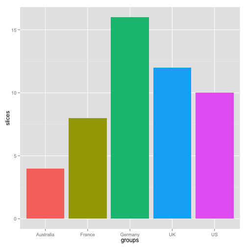
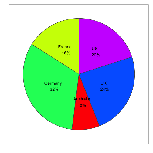
slices <- c(10, 12, 4, 16, 8)
groups <- c("US", "UK", "Australia", "Germany", "France")
pct <- paste(round(slices/sum(slices)*100),"%",sep="")
lbls <- paste(groups, "\n",pct) # add percents to labels
pie(slices,labels = lbls, col=rainbow(length(lbls)))

df_ex = data.frame(slices, groups, lbls, pct)
df_ex$fraction = df_ex$slices / sum(df_ex$slices)
df_ex$ymax = cumsum(df_ex$fraction)
df_ex$ymin = c(0, head(df_ex$ymax, n = -1))
# Pie / Donut plot
Pie = ggplot(data = df_ex, aes(fill = lbls, ymax = ymax, ymin = ymin, xmax = 4, xmin = 3)) +
    geom_rect(colour = "grey30", show_guide = FALSE) +
    coord_polar(theta = "y") +
 #   xlim(c(0, 4)) +
    theme_bw() +
    theme(panel.grid=element_blank()) +
    theme(axis.text=element_blank()) +
    theme(axis.ticks=element_blank()) +
    geom_text(aes(x = 3.5, y = ((ymin+ymax)/2), label = lbls)) +
    xlab("") +
    ylab("")+
     scale_fill_manual(values=rainbow(length(lbls)))
print(Pie)
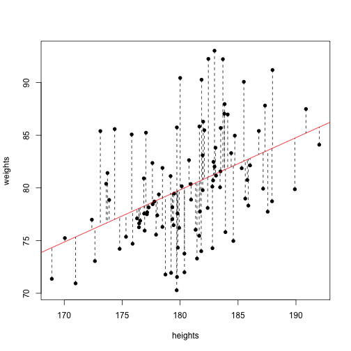
공분산(Covariacne)과 상관관계(Correlation)
- 두 변수의 변화 사이의 관계, 한 변수가 증가함에 따라 다른 변수가 변화하는 경향성
set.seed(1)
heights = rnorm(100,180,5)
heights = sort(heights, decreasing = F)
weights =  -10 + heights*.5 + rnorm(100,0,5)
#hist(weights);hist(heights)
cor(weights, heights)
## [1] 0.4214
## NULL
library("xtable")
print(xtable(coef(summary(lm(weights ~ heights)))),type="html")
| Estimate | Std. Error | t value | Pr(>|t|) | |
|---|---|---|---|---|
| (Intercept) | -9.40 | 19.46 | -0.48 | 0.63 |
| heights | 0.50 | 0.11 | 4.60 | 0.00 |
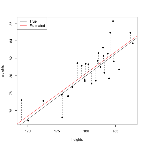
Regression
Least Squares
Function to minimize w.r.t \(b_{0}\), \(b_{1}\) \[ Q = \sum_{i=1}^{n}(Y_{i} - \hat{Y_{i}})^{2} = \sum_{i=1}^{n}(Y_{i} - (b_{0}+b_{1}X_{i}))^{2} \]
How to ? \[ \frac{dQ}{db_{0}} = 0 \] \[ \frac{dQ}{db_{1}} = 0 \]
## NULL
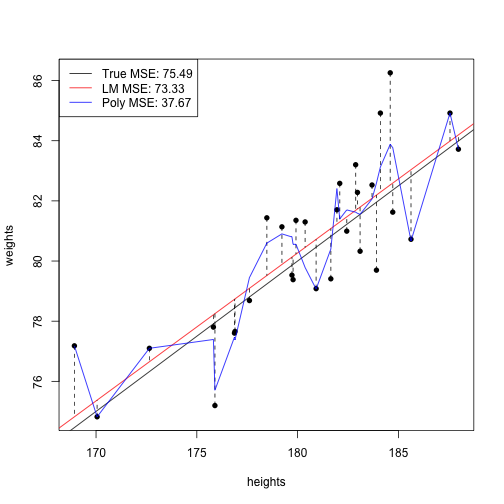
Over-Fitting(과적합)
## NULL
plot(heights, weights, pch=16)
abline(a=-10,b=.5,col="black")
abline(lm(weights ~ heights), col="red")
apply(cbind(heights, heights, weights, predict(lm(weights~heights))),1,
      function(coords){lines(coords[1:2],coords[3:4],lty=2)})

lm_mse = sum((weights - predict(lm(weights ~ heights)))^2)
true_mse = sum((weights - (-10 + .5*heights))^2)

poly_lm<-lm(weights ~ poly(heights,20))
points(heights,predict(poly_lm),type="l",col="blue")
poly_mse = sum((weights - predict(poly_lm))^2)

legend(170,93,legend=c(paste("True MSE:",round(true_mse,2)),
                       paste("LM MSE:",round(lm_mse,2)),
                       paste("Poly MSE:",round(poly_mse,2))),
              col=c("black","red","blue"),lty=1)